

A Dockerized RAG stack is a set of cooperating services rather than one application container. The web layer, ingestion workers, embedding service, vector database, model server, and supporting infrastructure each own a distinct stage of the data or query path. This article maps those containers, follows a document from upload to vector storage, and traces a user question through the six-step retrieval and generation flow.
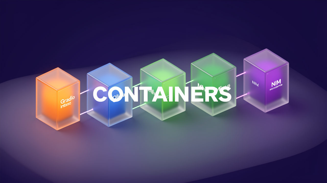
Reading docker ps stops being confusing the moment you compare compose files at different scales. The stacks I traced fall into a clear spectrum — a minimal three-container setup, an API-shaped four-service build, and an eight-container enterprise workflow — and the same roles keep reappearing in all of them.
The LlamaIndex Agentic RAG project is the smallest complete stack I mapped, and its compose.yaml starts exactly three services:
The maintainers are explicit about why Compose is required here: a single Dockerfile alone is not sufficient, because the app depends on several cooperating containers that need orchestration. The requirements stay modest — Linux and at least 8 GB of RAM — and the whole stack launches with docker compose up --build.
The RAG-LLM project takes a different shape. Its docker-compose.yml defines the full stack as Milvus + Redis + rag-api + a Celery worker, built from a multi-stage Dockerfile. But the compose file only tells half the story. A Client (Swagger UI) talks to the FastAPI application, and a RAGController inside it orchestrates the pipeline while connecting to three external components:
That last detail deserves a pause: in this stack, the LLM is not containerized at all. LM Studio runs as a standalone local server, and the API simply points at it through an OpenAI-compatible URL. The API itself is served by uvicorn on port 8081, with Swagger docs at http://localhost:8081/docs — a useful first stop for checking whether the stack is alive.
The NVIDIA AI Chatbots with RAG workflow is where docker ps starts reading like an inventory report:
rag-application-* — the chain server implementing ingestion and retrieval logicThe Multi-Turn RAG example adds an eighth container, nemo-retriever-reranking-microservice, which ranks the retrieved document chunks before they reach the LLM. In these deployments, that Milvus trio shows why the database does not ship as one image; it operates as a small distributed system.
The default models across the NVIDIA examples are meta/llama3-8b-instruct deployed on-prem via NIM, nv-embedqa-e5-v5 for embeddings, and the optional nv-rerankqa-mistral-4b-v3 for ranking. Prerequisites scale up accordingly: Docker, GPU driver 535+, the NVIDIA Container Toolkit, and an NGC API key. The docs even specify the command for verifying the deployment:
docker ps --format "table {{.ID}}\t{{.Names}}\t{{.Status}}"
Not every stack needs that much machinery. Docker's official RAG guide runs a Streamlit server service at http://localhost:8501, a Qdrant database service, and an optional Ollama service. A ChromaDB-based variant runs exactly four containers: ai_platform (Ollama), vector_db (ChromaDB), myragapp (the API backend — container name api-container, host port 6050), and react-ui.
Line these stacks up and the pattern is hard to miss. Every RAG deployment, from three containers to eight, is assembled from the same recurring roles: a UI layer, an API or chain server, an embedding service, an LLM server, and a vector store — plus infrastructure helpers like model pullers, task queues, object storage, and metadata stores. What differs is how many containers each role gets, and whether the LLM lives inside the compose file at all. Knowing the lineup answers what runs, though — not what happens. For that, the next stop is ingestion: how a raw PDF turns into searchable vectors.

A useful way to read the stack is to separate built images from borrowed images. The rule of thumb holds across every documented stack: you build images for code you own, and you pull images for infrastructure you rent. The FastAPI + LlamaIndex + Qdrant + Ollama pattern makes this concrete. Exactly two custom images are built — the API image (the FastAPI application) and the data ingestion tool image (the script that downloads, embeds, and loads documents into Qdrant) — while exactly two official images are pulled and run as-is: qdrant/qdrant and the prebuilt ollama/ollama:latest. Because the app needs a local LLM created from a custom Modelfile, a bash script copies the correct file and runs the created LLM — a piece of orchestration glue that lives between the images rather than inside them.
The mechanism behind this split is plain Compose semantics:
build key: services with a context like ./api plus a Dockerfile get their images built and tagged.image key: services specifying only an image are pulled from a registry if not found locally.One keyword, two completely different behaviors — and it explains why the borrowed half of your stack never needs a rebuild.
The Agentic RAG project builds just one custom image from its Dockerfile (the Gradio app) and pushes all model acquisition to runtime: an Ollama Pull service downloads the LLM model into the Ollama server once the containers are up. The maintainers openly warn that docker compose up --build takes a while, and the reason is instructive: pulling all the LLM models — not compiling code — is the time-consuming step.
One local stack bakes the pulls directly into the Ollama entrypoint:
ollama serve & starts the server in the background.sleep 5 gives it a moment to come up.ollama pull all-minilm fetches the embedding model.ollama pull qwen2:0.5b fetches the LLM.The matching healthcheck runs ollama list with a 30s interval, 10s timeout, 10 retries, and a 300s start_period — that generous start period exists specifically to absorb the initial model pulls before the container is declared healthy.
Two more details sharpen the picture. The data_ingestion service is deliberately excluded from default startup: docker compose up ollama qdrant api builds the base image, starts Qdrant and Ollama, then starts the API — while ingestion sits in the data-ingest Compose profile, run only on demand when documents actually need to be loaded. On the NVIDIA side, the split tilts almost entirely toward borrowing: the NIM and Milvus images come from nvcr.io, and Compose cannot fetch them until you run docker login nvcr.io with an NGC account and export NGC_API_KEY=<ngc-api-key>. The chain server is the single piece teams typically rebuild, since the workflow explicitly supports building and running a custom chain server.
Once I internalized this divide, docker ps stopped being noise: every entry was either my code or rented infrastructure, and I knew exactly which was which.
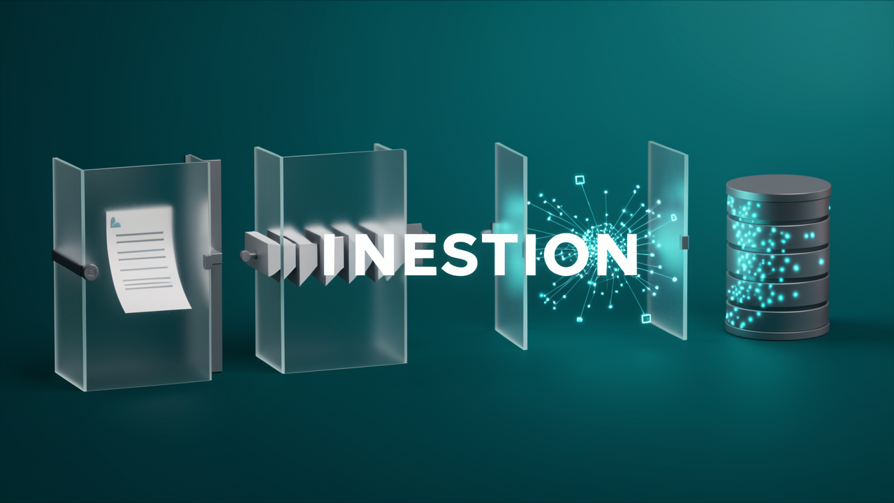
With the container map sorted out, the next thing I traced was what happens inside the stack when a document actually arrives. Every upload — PDF, TXT, or MD — walks the same four-stage pipeline, and once you can name those stages, the Celery and Milvus entries in your docker ps output start to feel intentional rather than decorative.
src/services/ingestion/chunker.py. This is the only stage where file types matter — after it, everything is plain text.RecursiveCharacterTextSplitter at 512 characters per chunk, with 128 characters of overlap between neighbors. A cleaning pass strips whitespace and special characters. That overlap is the detail I keep pointing people to: it stops a sentence from being severed at a chunk boundary and losing its context.MILVUS_HOST and MILVUS_PORT=19530. At this point, the document stops being a file and becomes searchable geometry.This is where the container count finally explains itself. Because large uploads are slow, the RAG-LLM stack runs ingestion asynchronously: the FastAPI API hands ingestion tasks to a Redis-backed Celery queue, and the Celery worker container consumes them — so a big PDF upload never blocks the query path. The compose file reflects that split:
docker-compose up -d rag-api — starts the API alone, valid when the Milvus/Redis infrastructure is already running.docker-compose up -d standalone redis — brings up infrastructure only.The NVIDIA chain server runs the identical journey, and its logs spell it out plainly:
INFO:example:Ingesting <file-name>.pdf in vectorDBINFO:RetrievalAugmentedGeneration.common.utils:Using milvus as vector storeBoth lines are driven by the chain-server environment variables APP_VECTORSTORE_NAME: "milvus" and APP_VECTORSTORE_URL: "http://milvus:19530" — the same port 19530 from my compose file, just written as a URL.
From there, the reference examples branch in ways worth knowing:
That last example is the reminder I needed: the four-stage pipeline is the standard path for unstructured text. Once your data arrives already structured, the embedding-and-vectorizing machinery becomes optional. For everything else, though, the pipeline ends the same way — with normalized vectors sitting in Milvus, waiting for a question.
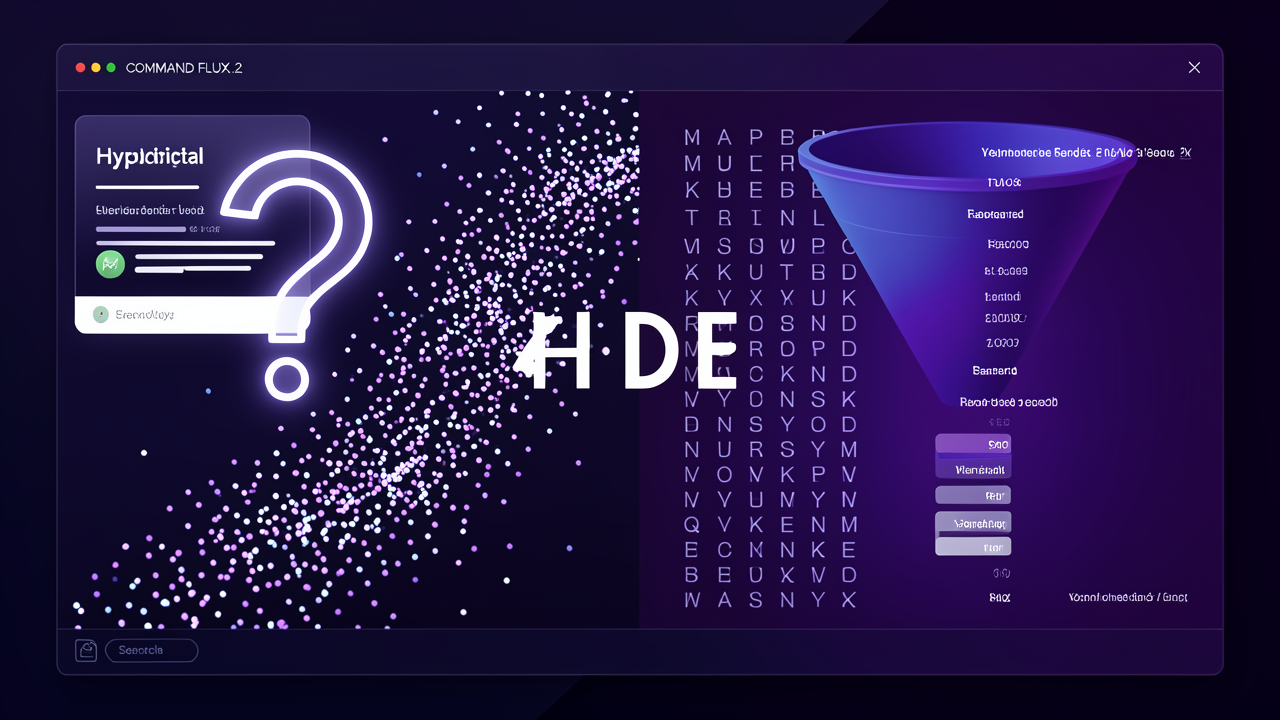
With the vectors already sitting in Milvus after ingestion, I expected the query path to be short: embed the question, fetch the nearest chunks, done. The RAGController had other plans. Its six-step pipeline opens with a detour through the LLM — and tracing that detour turned out to be one of the most instructive parts of the whole exercise.
Query enhancement lives in src/services/retrieval/hyde.py and implements HyDE (Hypothetical Document Embeddings). The sequence sounds backwards until you see why it works:
The reasoning is rooted in how embedding space behaves: questions and answers often live in different regions of that space, so a hypothetical document sits closer to real answers than the original question ever would. Retrieving with it improves recall of relevant passages.
Since HyDE costs an extra LLM call on every query, the stack ships with two levels of control:
ENABLE_HYDE — a global environment toggle, defaulting to true.enable_hyde — a per-request flag in the /query request body.This is also the first moment in the query flow where the app container hands work to the LLM server. The container I once couldn't explain in docker ps now has a clear job description: inventing an answer so the stack can search for the real one.
Step 2 lives in src/services/retrieval/hybrid_search.py and runs two parallel retrieval strategies before merging the results:
rank_bm25 library) for keyword-based term matching and exact keyword relevance. This leg works on terms rather than embeddings, so it's where exact wording wins.The two ranked lists are merged using Reciprocal Rank Fusion:
RRF(d) = Σ 1/(k + rank(d))
Each document's reciprocal ranks are summed across both result lists, with the constant k damping the difference between adjacent ranks. The effect: a document ranked highly by either strategy rises in the fused ranking — even if the other strategy barely noticed it.
The pairing is deliberate, and once I mapped it out, it stopped looking like over-engineering. Dense search misses exact keyword matches; BM25 misses semantically related phrasing. Each leg covers precisely the other's blind spot — and that complementarity is the entire point of running them in parallel before fusing their rankings.
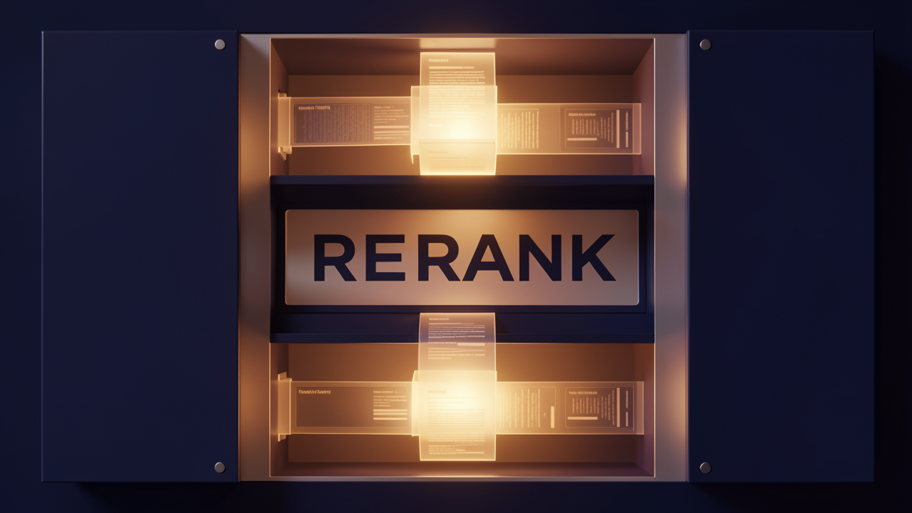
Hybrid search hands us 20 candidate chunks by default — but they're ordered by vector similarity, not by how well they actually answer the question. Those are not the same thing, and the next three steps of the flow exist precisely because of that gap.
The reranker lives in src/services/retrieval/reranker.py and runs a cross-encoder model: ms-marco-MiniLM-L-6-v2. The architectural choice matters here. The bi-encoder used during retrieval embeds the query and each passage independently and only compares vectors afterward — fast, but the two texts never influence each other's representation. A cross-encoder inverts that: it takes each (query, passage) pair as a joint input and scores the pair as a unit, which makes it far more accurate at judging true relevance.
Each candidate gets a real relevance score, the list is re-ordered by those scores, and only the top chunks survive to generation. The knobs controlling this:
That per-request flag is the detail I appreciate most: it lets you A/B the reranker's effect on answer quality without touching deployment config.
Before anything reaches the LLM, src/services/generator/prompt_optimizer.py applies two techniques — and neither of them involves a model call:
What stands out to me is the cost-benefit ratio: this step is pure text manipulation, costs nothing at inference time, and directly targets a documented LLM weakness.
Now the optimized context plus the original query travel to the LLM together with a grounding system prompt. In the RAG-LLM stack, that LLM server is LM Studio:
The generation endpoint supports SSE streaming, so answers render token by token in the client instead of arriving as one opaque block.
The NVIDIA workflow mirrors this shape with different plumbing: generation goes to the nemollm-inference-microservice, hosting the TensorRT-optimized meta/llama3-8b-instruct. And there's a symmetry worth noticing here — the optional reranking NIM, nv-rerankqa-mistral-4b-v3, plays exactly the same cross-encoder role in the Multi-Turn RAG example. Swap the stack, keep the step-3 logic.
That leaves one step in the six-step flow — the part that makes the answer sourced, not just fluent.

The sixth step is where the pipeline stops trusting its own output blindly. Self-RAG — the reflection stage — lives in src/services/generator/self_rag.py and works as the stack's built-in quality control. Before anything reaches the user, the LLM grades its own answer against two questions:
If confidence falls below the threshold, the answer is not returned as-is. A weak or unsupported draft triggers exactly one second attempt — and that attempt is smarter than a blind rerun.
Repeating the same generation with the same context would just reproduce the same weak answer, so the retry loop restructures the problem instead:
The design detail I find most practical here is the hard cap: a maximum of 1 retry, an explicit guard against infinite loops. If the second draft is still imperfect, it goes out anyway — one imperfect answer beats a pipeline stuck reflecting forever. That's a deliberate design stance, not an oversight.
Self-RAG targets a classic RAG failure: the right chunk was retrieved, but it ranked too low, so the model grounded its answer on the wrong evidence. Reranking in Step 3 fixes most of the ranking side before generation ever runs; Self-RAG is the safety net for whatever still slips through — the chunk that scored poorly but would have carried the answer.
When I look at where quality gains actually come from in a RAG flow, the pattern is consistent: production guidance ranks reranking and verification loops among the highest-ROI upgrades in the entire pipeline. The honest cost here is one extra LLM call whenever the first attempt is judged weak — a trade-off I'd accept in most production settings, because the alternative is silently shipping unsupported answers.
Like every other stage, Self-RAG follows the same configuration pattern:
And with that, all six steps are done. The pipeline returns a Final Answer plus Sources plus Metadata — which is exactly why responses from this stack arrive with citations attached rather than as a bare string. A raw question went in one end of the RAGController, and a grounded, sourced answer came out the other.
Once I could name every container in these stacks, one last pattern became impossible to miss: none of them is really a fixed set of services. The well-designed ones are menus. Compose profiles, separate override files, and request-level toggles decide what actually boots, which means the stack you run is the stack your use case needs — nothing more.
The NVIDIA workflow makes this explicit in its boot command:
USERID=$(id -u) docker compose --profile local-nim --profile milvus up -d
The local-nim profile brings the NIM containers; milvus brings the vector store and its dependencies. Leave a profile out and those services simply never start. The reranking microservice goes one step further and lives in a second file, deployed with USERID=$(id -u) docker compose -f docker-compose-nim-ms.yaml up -d ranking-ms — ranking is an add-on, not a core dependency, so the base pipeline works fine without it.
The lighter stacks use the same trick for ingestion. The data_ingestion service sits in the data-ingest profile and only runs when documents actually need to be embedded and loaded. It doesn't idle next to the query path; it appears, embeds, and stays out of docker ps the rest of the time.
The same workflow ships six example applications:
Structured Data RAG is the floor that proves the pattern: just rag-playground plus the rag-app-structured-data service. No embedding model, no vector database — PandasAI works directly over CSV dataframes. It also swaps the default llama3-8b-instruct for the larger meta/llama3-70b-instruct model, which Query Decomposition RAG uses as well. When your data is already structured, half the anatomy disappears.
Changing the vector store is not a rewrite. It means editing two chain-server environment variables — APP_VECTORSTORE_NAME and APP_VECTORSTORE_URL — then running docker compose down followed by up -d again. That is the whole operation, and the workflow supports Milvus, pgvector as the alternative vector database, Meta Llama 3 70B Instruct as the alternative LLM, and a custom chain server.
The RAG-LLM stack mirrors this philosophy at two levels. docker-compose up -d boots the full Milvus + Redis + API + Celery Worker stack, while docker-compose up -d rag-api starts only the API when the infrastructure is already running. The global toggles ENABLE_HYDE, ENABLE_RERANKING, and ENABLE_SELF_RAG then have per-request mirrors — enable_hyde, enable_reranking, enable_self_rag — so a caller can turn on HyDE for one difficult query and skip reranking for the simple ones. Quality becomes a per-request decision instead of a fixed property of the deployment.
What I appreciate most is that verification never changes across any of this. Whatever combination of profiles, files, and toggles I boot, the same two commands answer every question: docker ps for the inventory, and docker logs -f <rag-example> to watch the flow in real time. At this point, that inventory reads exactly the way I wanted it to on day one — like a table of contents.